摘要:使用Python实现数学建模中的一些常见算法和求解过程…
规划
线性规划
scipy求解
需要知道目标函数(一般是求最大或者最小值)和约束条件
求解前转化为下面的标准形式

1 | from scipy import optimize |
- 标准形式是<=,如果是>=,则在两边加上符号-
举例1
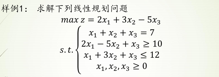
使用scipy求解z的最大值
c是目标函数的系数矩阵
A是化成标准的<=式子的左边的系数矩阵
B是化成标准的<=式子的右边的数值矩阵
Aeq是所有=左边的系数矩阵,记得里面是[[]]二维
Beq是所有=右边的数值矩阵
下面第11行-c加-,是因为此题求的是最大值,但是标准格式是求最小值,所以加负号
另外上面的3个变量都大于0,这里可以使用
bounds=(0, None),bounds=(min,max)是范围,None代表无穷,如果不写bounds,那默认是(0, None)1
res = optimize.linprog(-c, A, B, Aeq, Beq, bounds=(0, None))
1
2
3
4
5
6
7
8
9
10
11
12
13from scipy import optimize
import numpy as np
# 确定c,A,b,Aeq,beq
c = np.array([2, 3, -5])
A = np.array([[-2, 5, -1], [1, 3, 1]])
B = np.array([-10, 12])
Aeq = np.array([[1, 1, 1]])
Beq = np.array([7])
# 求解
res = optimize.linprog(-c, A, B, Aeq, Beq)
print(res)- res
1
2
3
4
5
6
7
8
9
10con: array([1.80713222e-09])
fun: -14.57142856564506
message: 'Optimization terminated successfully.'
nit: 5
slack: array([-2.24583019e-10, 3.85714286e+00])
status: 0
success: True
x: array([6.42857143e+00, 5.71428571e-01, 2.35900788e-10])
Process finished with exit code 0- fun是目标函数最小值
- x是最优解,即上面的x1,x2,x3的最优解
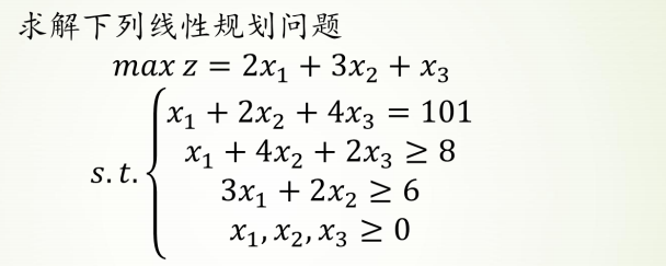
举例2
1 | from scipy import optimize |
1 | con: array([3.75850107e-09]) |
pulp求解
也可以使用pulp求解,见https://www.bilibili.com/video/BV12h411d7Dm?p=4
但是稍微繁琐
pymprog求解
举例
1 | maximize 15 x + 10 y # profit |
1 | from pymprog import * |
- res
1 | GLPK Simplex Optimizer, v4.65 |
整数规划
cvxpy求解
和线性规划差不多,但是多了个约束,那就是部分变量被约束为整数
目前没有一种方法可以有效地求解一切整数规划。常见的整数规划求解算法有:
- 分支定界法:可求纯或混合整数线性规划;
- 割平面法:可求纯或混合整数线性规划;
- 隐枚举法:用于求解0-1整数规划,有过滤隐枚举法和分支隐枚举法;
- 匈牙利法:解决指派问题(0-1规划特殊情形);
- Monte Carlo法:求解各种类型规划。
举例1

- 同理也是化成<=的标准形式
- 这里的改动只需要我们输入n,a,b,c,以及第10行的小改动,n,a,b,c含义和上面线性规划一样,如果有Aeq和Beq也是同理,加上即可,然后放进cons(下面第11行)里面
- 如果是求最大,第10行用cp.Maximize
1 | import cvxpy as cp |
- 运行结果会有警告,但是不影响结果
1 | 0: obj = 2.700000000e+02 inf = 6.250e-01 (1) |
非线性规划
非线性规划可分为两种,目标函数是凸函数或者是非凸函数
计算1/x+x的最小值
- 只需要改12行的系数,15行的初始猜测值,和8行的函数
- 如果结果是True,则是找到局部最优解,若是False,则结果是错误的
1
2
3
4
5
6
7
8
9
10
11
12
13
14
15
16
17
18
19
20
21from scipy.optimize import minimize
import numpy as np
# f = 1/x+x
def fun(args):
a = args
return lambda x: a / x[0] + x[0]
if __name__ == '__main__':
args = (1) # a
# x0 = np.asarray((1.5)) # 初始猜测值
# x0 = np.asarray((2.2)) # 初始猜测值
x0 = np.asarray((2)) # 设置初始猜测值
res = minimize(fun(args), x0, method='SLSQP')
print('最值:', res.fun)
print('是否是最优解', res.success)
print('取到最值时,x的值(最优解)是', res.x)1
2
3
4
5最值: 2.00000007583235
是否是最优解 True
取到最值时,x的值(最优解)是 [1.00027541]
Process finished with exit code 0
举例2

x1,x2,x3的范围都在0.1到0.9 之间
x是变量矩阵,如x[0]即为x1
需要变动的是函数fun,con,27,29,32行,x0的设置要尽在要求的0.1到0.9范围内
1
2
3
4
5
6
7
8
9
10
11
12
13
14
15
16
17
18
19
20
21
22
23
24
25
26
27
28
29
30
31
32
33
34
35
36
37from scipy.optimize import minimize
import numpy as np
# 计算(2+x1)/(1+x2)- 3*x1+4*x3
def fun(args):
a, b, c, d = args
return lambda x: (a + x[0]) / (b + x[1]) - c * x[0] + d * x[2]
def con(args):
# 约束条件 分为eq 和ineq
# eq表示 函数结果等于0
# ineq 表示 表达式大于等于0
x1min, x1max, x2min, x2max, x3min, x3max = args
cons = ({'type': 'ineq', 'fun': lambda x: x[0] - x1min},
{'type': 'ineq', 'fun': lambda x: -x[0] + x1max},
{'type': 'ineq', 'fun': lambda x: x[1] - x2min},
{'type': 'ineq', 'fun': lambda x: -x[1] + x2max},
{'type': 'ineq', 'fun': lambda x: x[2] - x3min},
{'type': 'ineq', 'fun': lambda x: -x[2] + x3max})
return cons
if __name__ == "__main__":
# 定义常量值
args = (2, 1, 3, 4) # a,b,c,d
# 设置参数范围/约束条件
args1 = (0.1, 0.9, 0.1, 0.9, 0.1, 0.9) # x1min, x1max, x2min,x2max
cons = con(args1)
# 设置初始猜测值
x0 = np.asarray((0.5, 0.5, 0.5))
res = minimize(fun(args), x0, method='SLSQP', constraints=cons)
print('最值:', res.fun)
print('是否是最优解', res.success)
print('取到最值时,x的值(最优解)是', res.x)1
2
3
4
5最值: -0.773684210526435
是否是最优解 True
取到最值时,x的值(最优解)是 [0.9 0.9 0.1]
Process finished with exit code 0可以看出对于这类简单函数,局部最优解与真实最优解相差不大,但是对于复杂的函数,x0的初始值设置,会很大程度影响最优解的结果
数值逼近
一维和二维插值
- 参考https://www.bilibili.com/video/BV12h411d7Dm?p=5
- 都使得图像更加光滑
最小二乘法拟合
用的是
1
from scipy.optimize import leastsq
举例
一组数据:
1
2X = np.array([8.19, 2.72, 6.39, 8.71, 4.7, 2.66, 3.78])
Y = np.array([7.01, 2.78, 6.47, 6.71, 4.1, 4.23, 4.05])使用leastsq
1 | import numpy as np |
1 | k = 0.6134953491930442 |

另外,这个线性拟合也可以使用sklearn求k和b,再去画图
- 注意维度转换X = X.reshape(-1, 1)
1
2
3
4
5
6
7
8
9
10
11
12
from sklearn import linear_model
import numpy as np
if __name__ == '__main__':
X = np.array([8.19, 2.72, 6.39, 8.71, 4.7, 2.66, 3.78])
Y = np.array([7.01, 2.78, 6.47, 6.71, 4.1, 4.23, 4.05])
X = X.reshape(-1, 1)
model = linear_model.LinearRegression()
model.fit(X, Y)
print('k = ', model.coef_)
print('b = ', model.intercept_)1
2
3
4k = [0.61349535]
b = 1.7940925542916233
Process finished with exit code 0更多线性和非线性问题、如多元回归、逻辑回归、其他分类问题,见我之前的sklearn blog
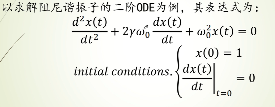
微分方程
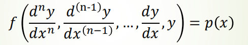
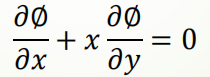
微分方程是用来描述某一类函数与其导数之间关系的方程,其解是一个符合方程的函数。微分方程按自变量个数可分为 常微分方程和偏微分方程,
前者表达通式 :
后者表达通式:
建议稍微复习一下高数上册最后微分方程那章再看看会更好
解析解
使用sympy库,但是得到的是字符形式的格式
如下这种,如果结果是比较复杂的,可能太丑
如
1
2
3
4
5
6
7
8
9
10
11
12
13
14
15
16
17
18
19import sympy
def apply_ics(sol, ics, x, known_params):
free_params = sol.free_symbols - set(known_params)
eqs = [(sol.lhs.diff(x, n) - sol.rhs.diff(x, n)).subs(x, 0).subs(ics) for n in range(len(ics))]
sol_params = sympy.solve(eqs, free_params)
return sol.subs(sol_params)
if __name__ == '__main__':
sympy.init_printing() # 初始化打印环境
t, omega0, gamma = sympy.symbols("t, omega_0, gamma", positive=True) # 标记参数,且均为正
x = sympy.Function('x') # 标记x是微分函数,非变量
ode = x(t).diff(t, 2) + 2 * gamma * omega0 * x(t).diff(t) + omega0 ** 2 * x(t)
ode_sol = sympy.dsolve(ode) # 用diff()和dsolve得到通解
ics = {x(0): 1, x(t).diff(t).subs(t, 0): 0} # 将初始条件字典匹配
x_t_sol = apply_ics(ode_sol, ics, t, [omega0, gamma])
sympy.pprint(x_t_sol)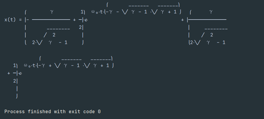
如果最后加上
print(x_t_sol)结果为:
1
2Eq(x(t), (-gamma/(2*sqrt(gamma**2 - 1)) + 1/2)*exp(omega_0*t*(-gamma - sqrt(gamma - 1)*sqrt(gamma + 1))) + (gamma/(2*sqrt(gamma**2 - 1)) + 1/2)*exp(omega_0*t*(-gamma + sqrt(gamma - 1)*sqrt(gamma + 1))))
结果较为简单的常微分方程
- f(x)’’+f(x)=0 二阶常系数齐次微分方程
1
2
3
4
5
6
7
8
9
10
11
12
13import sympy as sy
# f(x)''+f(x)=0 二阶常系数齐次微分方程
def differential_equation(x, f):
return sy.diff(f(x), x, 2) + f(x)
if __name__ == '__main__':
x = sy.symbols('x') # 约定变量
f = sy.Function('f') # 约定函数
print(sy.dsolve(differential_equation(x, f), f(x))) # 打印
sy.pprint(sy.dsolve(differential_equation(x, f), f(x))) # 漂亮的打印1
2
3
4Eq(f(x), C1*sin(x) + C2*cos(x))
f(x) = C₁⋅sin(x) + C₂⋅cos(x)
Process finished with exit code 0可以参考:https://blog.csdn.net/your_answer/article/details/79234275
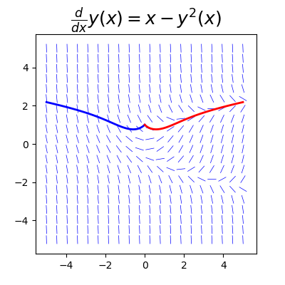
数值解
- 当ODE(常微分方程)无法求得解析解时,可以用scipy中的integrate.odeint求数值解来探索其解的部分性质,并辅以可视化,能直观地展现ODE解的函数表达
举例
一阶非线性常微分方程

plot_direction_field函数里面的参数意义:
- y_x:也就是y(x)
- f_xy:也就是x-y(x)^2
- x_lim=(-5, 5), y_lim=(-5, 5)也就是在这个x,y轴的范围展示出来
关键需要修改的部分,29-31行,33行的y0需要适当调
1
2
3x = sympy.symbols('x')
y = sympy.Function('y')
f = x - y(x) ** 2
1 | import numpy as np |
传染病模型
传染病模型研究属于传染病动力学研究方向,这里只是将模型中微分方程进行了python实现
传染病模型包括:SI、SIS、SIR、SIRS、SEIR、SEIRS共六个模型
SI模型
比如病毒传染初期,没有加防疫手段,就符合SI模型
SI模型的表达式见网上(S:易感染,I:已感染)
需要修改的参数
1
2
3
4
5
6N = 10000 # N为人群总数
beta = 0.25 # β为传染率系数
gamma = 0 # gamma为恢复率系数
I_0 = 1 # I_0为感染者的初始人数
S_0 = N - I_0 # S_0为易感染者的初始人数
T = 150 # T为传播时间- β为传染率系数,比如现在100个人已经传染了,在一段时间内,传染新增了25人,则β为0.25
- gamma为恢复率系数,一开始没有抗体都是为0的,如果不为0,比如是开始有100人感染,在一个传播时间T后,治愈了6个人,则gamma取0.06
- I_0为感染者的初始人数
- S_0为易感染者的初始人数,这个要看情况,如果都不加干预,那就是N - I_0,一般看情况需要再考虑其他因素(交通,社交群体,航线等),S_0考虑的越多,则越完备
- Susceptible易感染的,Infection已经感染的
code
1 | import numpy as np |

- 可以看到10000个人大概在60天左右就全部感染了
SIS模型
- 与SI区别不大,区别在于7行的gamma有初始值,以及17行的公式改变了
1 | import numpy as np |
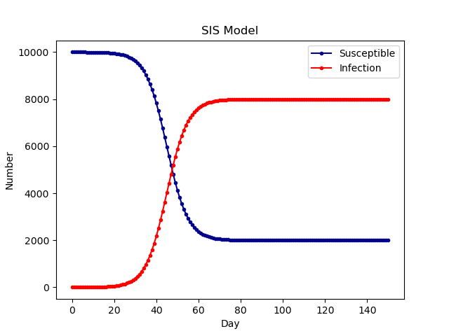
- 可以看到60-80天之间,逐渐稳定,有的人治愈后(获得抗体)活了下来,有的没治愈的就死了
SIR模型
- 多了R_0为治愈者的初始人数,即刚开始注射疫苗恢复的人
- 表达式也改变
- 注意恢复治愈包括自身产生抗体以及通过医疗手段获得抗体两种
1 | import numpy as np |

- 可以看到感染人数出现峰值,在前期已经开始使用抗体,病人逐渐治愈,最后所有人都恢复健康
SIRS模型
- 多了Ts为抗体持续时间,也就是说有了抗体一段时间后,抗体失效,又变成了易感染人群
- 公式也改变
1 | import numpy as np |
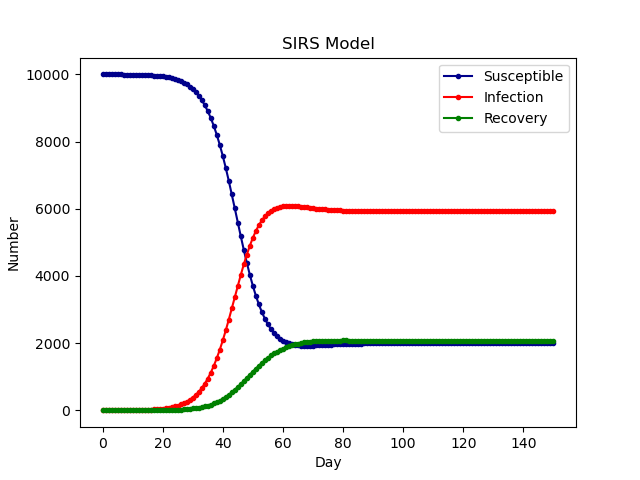
- 最终达到一个平衡
SEIR模型
考虑了病毒的潜伏期(潜伏人群E),也就是感染病毒后,过了潜伏期就是感染人群了
多了E_0为潜伏者的初始人数,如果是0,那说明开始时有人感染,但是还没有发病,此时这类人不是易感染,但是他们携带病毒
只有经过潜伏期,才能被传染
公式有所变化
1 | import numpy as np |
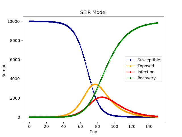
- 潜伏期的人会比感染人群先到达峰值,最终都可以治愈
SEIRS模型
考虑了抗体持续时间
一般多了潜伏期的话,传染率系数会有所增加,上面的SEIR也是同理
1 | import numpy as np |
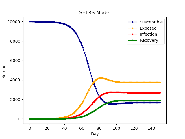
- 潜伏期的人先到峰值,然后是易感染者,然后是治愈者,他们最终会达到平衡稳定
图论
Dijkstra
解法1(常用)
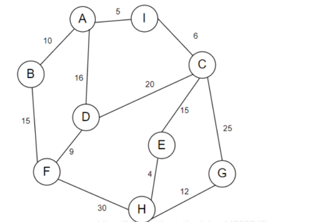
- 只需要给出带有权值的邻接矩阵即可求出最短路径和最短距离
- 需要改变的第54行邻接矩阵的权值和65行的起点和终点,注意21行是从0还是1开始
- 有向边和无向边的混合均可使用
g = defaultdict(list)是得到一个元素全是list类型的字典- 举例
1 | # dijkstra |
1 | 最短距离为:8 |
解法2
- 输入是一个包含每个点与其他点联系和权值的字典
- 下面是无向边的例子,适合无向边
- 需要修改的是51的联系,62的起点,66行的起点和终点
1 | import heapq |
1 | 该点的上一个点: {'A': None, 'B': 'A', 'D': 'A', 'I': 'A', 'C': 'I', 'F': 'B', 'E': 'C', 'H': 'E', 'G': 'H'} |
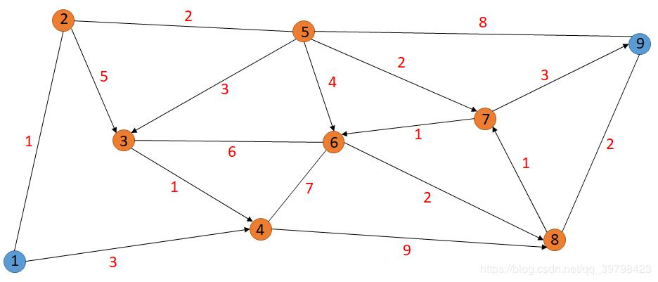
Floyd
- 通过动态规划求解多源最短路径问题
举例
- 图和上面的图一样,求出从每一个点到其他点的最短距离和路径
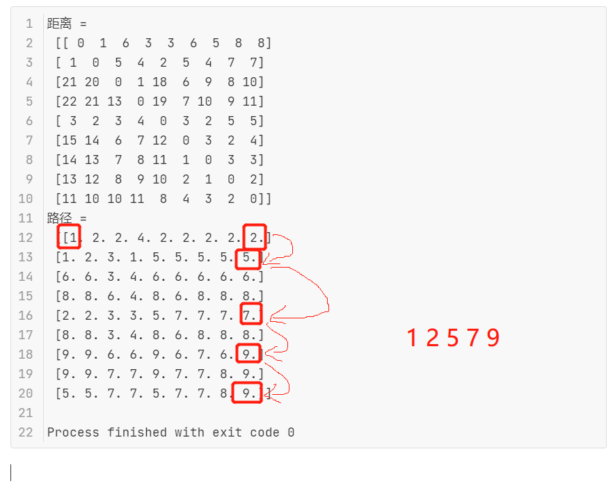
1 | import numpy as np |
1 | 距离 = |
距离,比如1到9的距离为8,即从第1行看到第9列
怎么看最短路径看解释见下图
机场航线设计
- 图的可视化
- 数据清洗分析,可参考我那块Kaggle练习
- 城市可作为图节点
- 可参考down下来的pdf资料
- 找到最密集的点,作为交通枢纽,考虑其他成本、时效性、盈利因素之类的…
回归
- 多元回归、逻辑回归见我之前的blog
- 也可参考pdf资料
差分方程
递推关系
- 差分方程建模的关键在于如何得到第n组数据与第n+1组数据之间的关系
举例
酵母菌生长模型
相类比的还有比如兔子(其他生物)繁殖模型等
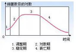
如图所示我们用培养基培养细菌时,其数量变化通常会经历这四个时期。
这个模型针对前三个时期建一个大致的模型:
调整期、对数期、稳定期
数据可以也从文件读入,这里直接写了
1
2
3
4
5
6
7
8
9
10
11
12
13
14import matplotlib.pyplot as plt
if __name__ == '__main__':
time = [i for i in range(0, 19)]
number = [9.6, 18.3, 29, 47.2, 71.1, 119.1, 174.6,
257.3, 350.7, 441.0, 513.3, 559.7, 594.8,
629.4, 640.8, 651.1, 655.9, 659.6, 661.8]
plt.title('Relationship between time and number') # 创建标题
plt.xlabel('time') # X轴标签
plt.ylabel('number') # Y轴标签
plt.scatter(time, number)
plt.plot(time, number) # 画图
plt.show() # 显示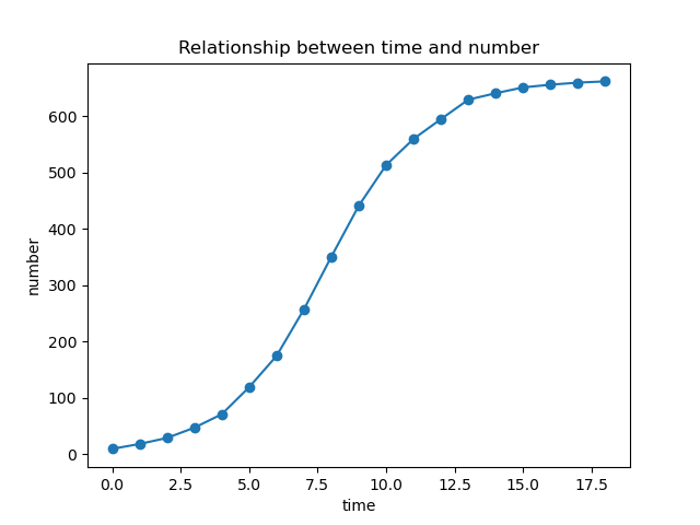
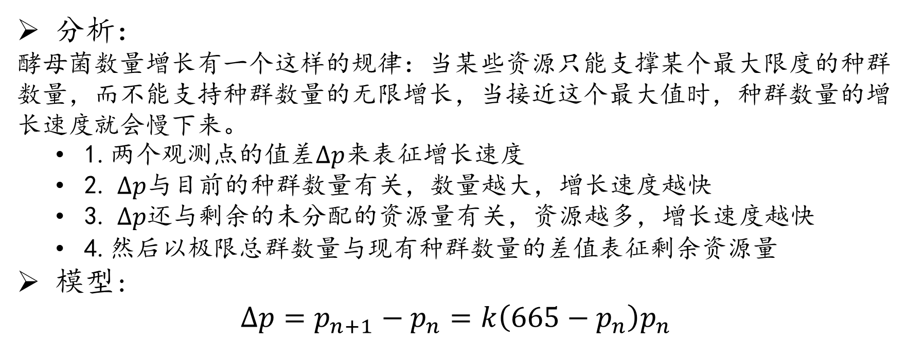
- Δp:因为横坐标间隔是1,所以相邻纵坐标之差可以当成增速
- 665是极限总群数量
- 要求的是k,然后预测下一年
- 需要修改的是4,17,18行,如果不只是算下一年,那要改40,46行
1 | import matplotlib.pyplot as plt |
1 | [ 0.00081448 -0.30791574] |

显式差分
马尔科夫链
选举投票预测
马尔科夫链是由具有以下性质的一系列事件构成的过程:
一个事件有有限多个结果,称为状态,该过程总是这些状态中的一个;
在过程的每个阶段或者时段,一个特定的结果可以从它现在的状态转移到任何状态,或者保持原状;
每个阶段从一个状态转移到其他状态的概率用一个转移矩阵表示,矩阵每行的各元素在0到1之间,每行的和为1。
选举投票趋势预测
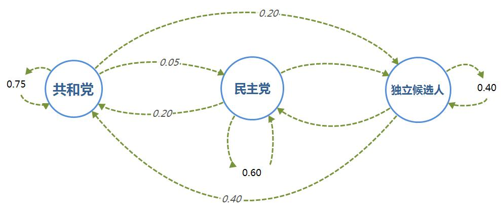
以美国大选为例,首先取得过去十次选举的历史数据,然后根据历史数据得到选民意向的转移矩阵,转移矩阵如下
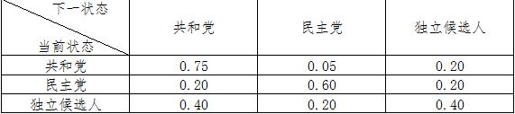
比如,当前状态的共和党转移到下一状态的共和党的概率是0.75,以此类推
即如下关系:
然后我们可以构造出差分表达式(共和党R,民主党D,独立候选人I):
也就是下个状态等于前一个状态的所有可能之和
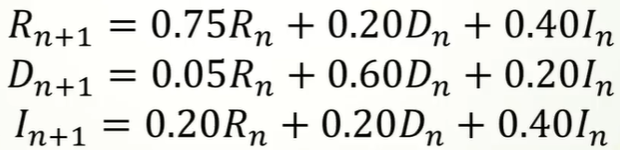
通过求解差分方程组,预测出选民投票意向的长期趋势
plt.annotate是标记文本,如
xy 1
2
3
4
5
6
7
8
9
10
11
12
13
14
15
16
17
18
19
20
21
22
23
24
25
26
27
28
29
```python
import matplotlib.pyplot as plt
if __name__ == '__main__':
RLIST = [1 / 3]
DLIST = [1 / 3]
ILIST = [1 / 3]
for i in range(40):
R = RLIST[i] * 0.75 + DLIST[i] * 0.20 + ILIST[i] * 0.40
RLIST.append(R)
D = RLIST[i] * 0.05 + DLIST[i] * 0.60 + ILIST[i] * 0.20
DLIST.append(D)
I = RLIST[i] * 0.20 + DLIST[i] * 0.20 + ILIST[i] * 0.40
ILIST.append(I)
plt.plot(RLIST)
plt.plot(DLIST)
plt.plot(ILIST)
plt.xlabel('Time')
plt.ylabel('Voting percent')
plt.annotate('DemocraticParty', xy=(5, 0.2))
plt.annotate('RepublicanParty', xy=(5, 0.5))
plt.annotate('IndependentCandidate', xy=(5, 0.25))
plt.show()
print(RLIST, DLIST, ILIST)
print('预测的最后一年:RLIST: {}, DLIST: {}, ILIST: {}'.format(RLIST[-1], DLIST[-1], ILIST[-1]))
遍历画出每一年,这是最后一年的图
1
2
3
4
5......
......
预测的最后一年:RLIST: 0.5555555555483689, DLIST: 0.1944444444516318, ILIST: 0.2500000000000002
Process finished with exit code 0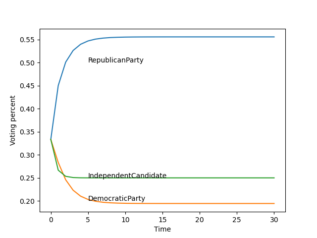
最后得到的长期趋势是:
56%的人选共和党、
19%的人选民主党、
25%的人选独立候选人
灰色与模糊
多层模糊评价
- 见资料
模糊c均值聚类
- 原理见资料
- 聚类的算法实现参考我之前sklearn里面的聚类算法实现就行了
灰色预测(经典常用)
灰色预测是用灰色模式GM(1,1)来进行定量分析的,通常分为以下几类:
灰色时间序列预测。用等时距观测到的反映预测对象特征的一系列数量(如产量、销量、人口数量、存款数量、利率等)构造灰色预测模型,预测未来某一时刻的特征量,或者达到某特征量的时间。
畸变预测(灾变预测)。通过模型预测异常值出现的时刻,预测异常值什么时候出现在特定时区内。
波形预测,或拓扑预测,通过灰色模型预测事物未来变动的轨迹。
系统预测,对系统行为特征指标建立一族相互关联的灰色预测理论模型,在预测系统整体变化的同时,预测系统各个环节的变化。
上述灰色预测方法的共同特征是:
允许少数据预测;
允许对灰因果律实践进行预测,例如:
灰因白果律事件:粮食生产预测(就是结果产量是已知的,中间受什么因素影响是未知的)
白因灰果律事件:开放项目前景预测(过程已知,但是结果前景未知)
具有可检验性(事前检验:建模可行性级比检验;模型检验:建模精度检验;
预测检验:预测滚动检验)
- 模型理论部分见资料或者网上看
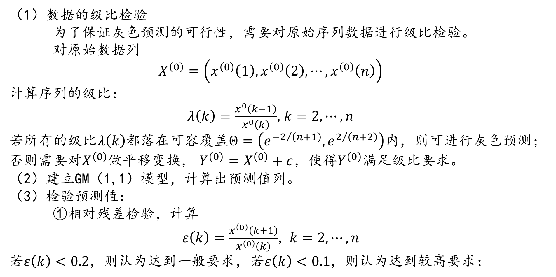
算法步骤
要使用灰色预测模型,首先看看适不适用
如果级比都落在可容覆盖范围内,就直接用
否则做平移变换

- 代码部分是可以使用cuda加速的
- 只需改87行的输入数据和93行的预测个数m
1 | import torch as th |
1 | <class 'numpy.ndarray'> |
蒙特卡罗
蒙特卡罗算法
由冯.诺依曼提出来的
蒙特·卡罗(Monte Carlo method)又称统计模拟方法,一种以概率统计理论为指导的数值计算方法。是指使用随机数(或者伪随机数)来解决很多计算问题的方法。
基本思想
当所求解问题是某种随机事件出现的概率,或者是某个随机变量的期望值时,通过某种“实验”的方法,以这种事件出现的频率估计这一随机事件的概率,或者得到这个随机变量的某些数字特征,并将其作为问题的解。
举例
蒙特卡罗方法求圆周率
基本思想:在图中区域产生足够多的随机数点,然后计算落在圆内的点的个数与总个数的比值再乘以4,就是圆周率。
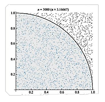
random.random()得到的是0到1之间的(伪)随机数,若要某个整数范围,则用random.randint(a, b),是有包括a和b的
1 | import math |
1 | 请输入一个较大的整数9999999 |
蒙特卡罗求定积分
利用python计算函数y=x**2在[0,1]区间的定积分
基本思想:和上例相似

1 | """ |
1 | 请输入一个较大的整数:999999 |
三门问题
背景
三门问题(Monty Hall probelm)亦称为蒙提霍尔问题,出自美国电视游戏节目Let’s Make a Deal。参赛者会看见三扇关闭了的门,其中一扇的后面有一辆汽车,选中后面有车的那扇门可赢得该汽车,另外两扇门则各藏有一只山羊。当参赛者选定了一扇门,但未去开启它的时候,节目主持人开启剩下两扇门的其中一扇,露出其中一只山羊。主持人其后问参赛者要不要换另一扇仍然关上的门。问题是:换另一扇门是否会增加参赛者赢得汽车的几率?如果严格按照上述条件,即主持人清楚地知道,自己打开的那扇门后面是羊,那么答案是会。不换门的话,赢得汽车的几率是1/3,换门的话,赢得汽车的几率是2/3
应用蒙特卡罗重点在使用随机数来模拟类似于赌博问题的赢率问题,通过多次模拟得到所要计算值的模拟值
解决思路:
在三门问题中,用0、1、2分代表三扇门的编号,在[0,2]之间随机生成一个整数代表奖品所在门的编号prize,再次在[0,2]之间随机生成一个整数代表参赛者所选择的门的编号guess。用变量change代表游戏中的换门(true)与不换门(false)

1 | import random |
1 | 玩100000次,每一次都换门: |
巧克力豆问题
- 见资料
时间序列
时序问题也可使用神经网络里面的LSTM(长短时记忆)
预测的是近期的,不是预测长远的(长远预测需要挖掘更多特征,深度学习那块的)
均方差:
1
2
3
4from sklearn.metrics import mean_squared_error
from math import sqrt
rms = sqrt(mean_squared_error(test, pred))# 把实际和预测的放进去
print(rms)
简单指数平滑法
- 导入数据
- 切分数据
- 代码适当修改和测试
1 | from statsmodels.tsa.api import SimpleExpSmoothing |
霍尔特线性趋势法
考虑到数据集变化趋势的方法就叫做霍尔特线性趋势法,任何呈现某种趋势(比如商上升趋势)的数据集都可以用霍尔特线性趋势法用于预测
先看看是否呈现某种趋势
1
2
3import statsmodels.api as sm sm.tsa.seasonal_decompose(train['xxx']).plot()
result = sm.tsa.stattools.adfuller(train['xxx'])
plt.show()- 如果是的话就可以使用
代码相对上面只需改动这两句,其他适当改即可
1 | from statsmodels.tsa.api import Holt |
Holt-Winters季节性预测模型
- 体现在季节性
- 比如一个水果店的销售情况,在夏季收入远高于其他季节
- 只需改变一点代码,选择了seasonal_period=7作为每周重复数据
1 | from statsmodels.tsa.api import ExponentialSmoothing |
自回归移动平均模型(ARIMA)
- 指数平滑模型都是基于数据中的趋势和季节性的描述,而自回归移动平均模型的目标是描述数据中彼此之间的关系。ARIMA的一个优化版就是季节性ARIMA。它像Holt-Winters季节性预测模型一样,也把数据集的季节性考虑在内。
1 | import statsmodels.api as sm |
时间序列最后都要评估一下
SVM
- 见之前的资料sklearn
1 | clf = svm.SVC(C=0.8, kernel='rbf', gamma=20, decision_function_shape='ovr') |
调参,参数见资料